August 20, 2016 / by / In , ,

Segmenting the Brachial Plexus with Deep Learning tl;dr: We competed in an image segmentation contest on Kaggle and finished 17th. Here is an overview of our approach.

Every summer our department hosts several summer interns who are considering graduate studies in biomedical informatics. This summer I had the great pleasure of supervising Ben Kompa who worked on several projects, including a Kaggle contest where we were challenged to detect and segment the brachial plexus in ultrasound images. This being a contest involving images, our approach naturally centered on the use of deep convolutional neural networks. It ended up being a close contest and we landed in the 17th spot of 923 teams and were within ~3% of the top teams. We had a lot of fun and learned a lot during the contest. Below is an overview of our experience.

Overview

The goal of the contest was to predict which pixels of an ultrasound image contain the brachial plexus. The contest is reflective of a larger trend in which AI (mostly deep learning) is starting to be used in radiology to automate some tasks. Indeed, Kaggle has had a few medical image challenges recently, so I expect this trend will continue for the foreseeable future.

For this challenge, we were given 5,635 training images (as 420x580 .tiffs) where the brachial plexus had been annotated by a person and we had to predict the pixel-by-pixel location of the brachial plexus for 5,508 testing images. In other words, this was an image segmentation challenge where the pixels in each image belonged to one of two possible classes: nerve vs. not nerve. Our task was to predict which of the possible 243,600 pixels were part of the brachial plexus for each image in the test set. Agreement between actual and predicted masks was measured using a modified form of the Dice coefficient. To be concrete, let be the binary vector representing the true mask for image and be the binary vector representing our predictions for image , where pixels. The Dice coefficient for is defined as:

where is the number of pixels where are both equal to 1 and is the total number of positive pixels in each vector. Note that .

However, there were a lot of images (more than half) where the brachial plexus was not present at all (i.e. is all 0s), or was not thought to be present by the person who annotated the image (more on this later). Because of this, the contest actually used a modified version of the Dice coefficient that gave a perfect score of 1 if you predicted an empty mask and were correct. The actual score metric was thus:

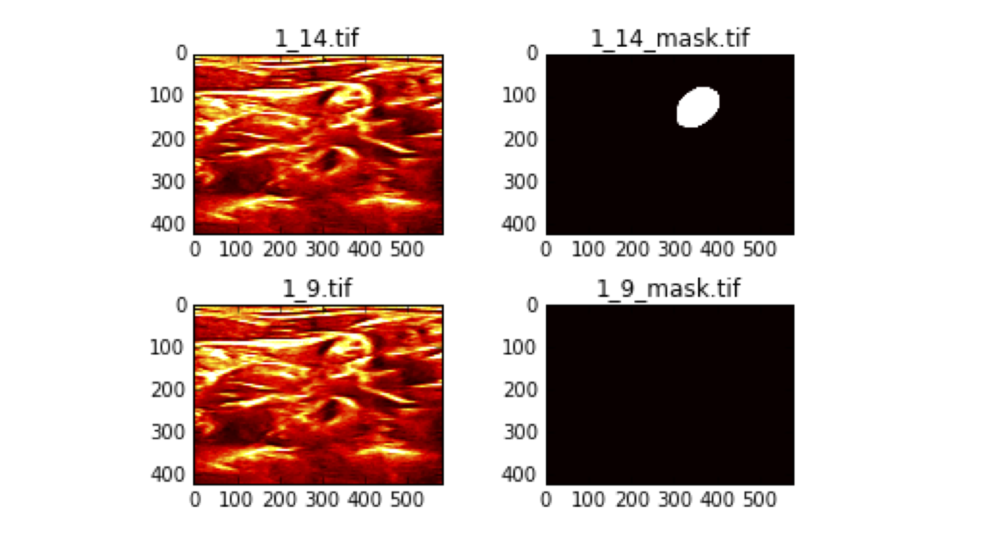
Outside of this unique scoring metric, there were a few data quality issues that were discovered during the course of the contest. For instance, some competitors noticed that several of the training images appeared to have been mislabeled. Below is a representative example.

These are two images from the same patient (“1_” indicates that these are both from patient 1), that look very similar yet have completely different annotations. Annotation 1_14_mask.tif shows the brachial plexus is present in the upper right-hand corner indicated by the white circle, while 1_9_mask.tif says that it is not present at all, despite the fact that there is very little visible different between the two ultrasound images (shown on the left). This meant that the task was more like “predict what an annotator probably saw” instead of “segment the brachial plexus”.

Approach

Our final approach ended up being relatively straightforward and was designed to reduce the variance we observed in our predictions. We fit a UNET model that minimized the negative log of a smooth version of the Dice coefficient, shown below:

where is the vector of probabilities for each pixel produced by the neural network. Note that if and , then the loss = 0 (i.e. the score = 1), so this gives us a nice, smooth approximation to the contest score function.

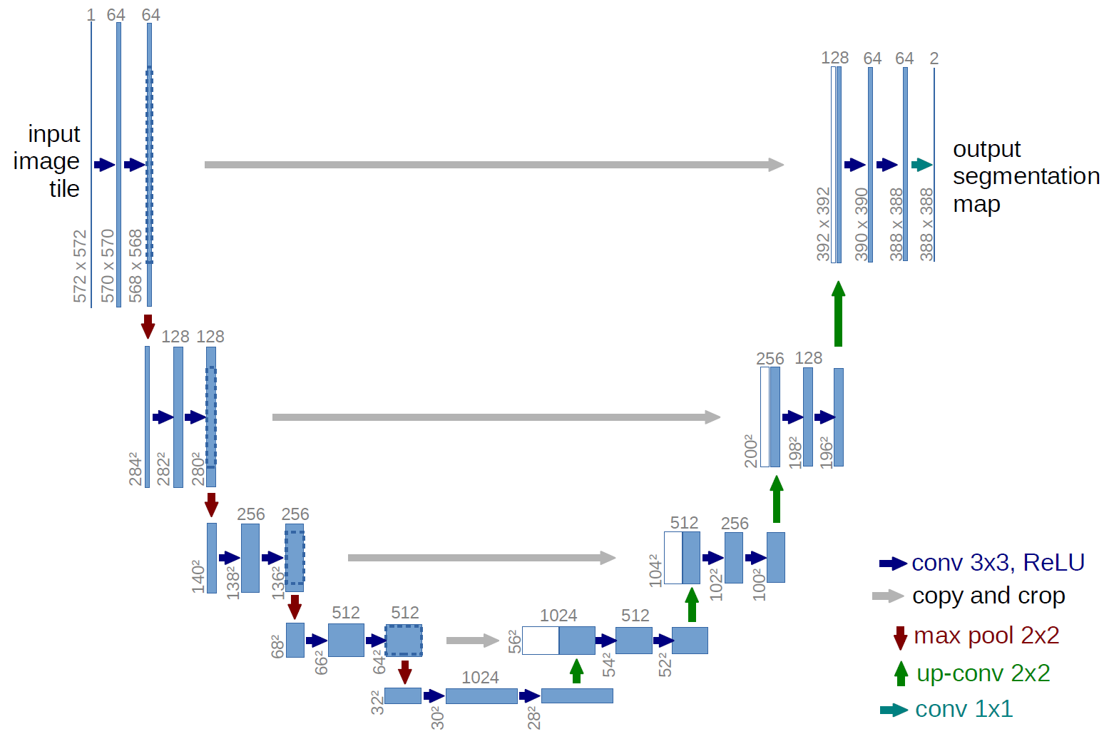
Our model was based in part on Marko Jocic’s Keras implementation. The UNET model has seen some success in image segmentation challenges (including 3rd place in the recent Data Science Bowl) and I suspect many other top teams were also using some form of the UNET. The main idea is that after each convolutional block, information travels along two pathways. One way is down a traditional down-sampling/max-pooling path that you would see in most CNNs and the other is a skip-type connection that merges with a convolutional block of the same volume, that is the result of an up-sampling path. A schematic of this from the UNET paper is shown below:

We fit models on various image sizes (64x80, 128x160, 192x240, and 256x320) and found, in general, larger images led to slightly better scores. All images were z-scored using the mean and standard deviation of the training set. We made a few important tweaks to the network such as using batch normalization on the down-sampling path and added dropout to each merge on the up-sampling path, and used the following data augmentations:

Horizontal and vertical flips

Horizontal and vertical shifts

Rotations

Shears

Zooms