February 23, 2017 / by / In

Deep Learning 101 - Part 2: Multilayer Perceptrons

tl;dr: What to do when you have standard tabular data. This post covers the basics of standard feed-forward neural nets, aka multilayer perceptrons (MLPs)

The Deep Learning 101 series is a companion piece to a talk given as part of the Department of Biomedical Informatics @ Harvard Medical School ‘Open Insights’ series. Slides for the talk are available here and a recording is also available on youtube

Other Posts in this Series Introduction

In this post we’ll cover the fundamentals of neural nets using a specific type of network called a “multilayer perceptron”, or MLP for short. The post will be mostly conceptual, but if you’d rather jump right into some code click over to this jupyter notebook. This post assumes you have some familiarity with basic statistics, linear algebra, calculus and python programming.

MLPs are usually employed when you have what most people would consider “standard data”, e.g. data in a tabular format where rows are samples and columns are variables. Another import feature here is that the rows and columns are both exchangeable, meaning we can swap both the order of the rows or the order of the columns and not change the ‘meaning’ on the input data.

MLPs are actually not responsible of most recent progress in deep learning, so why start with them instead of more advanced, state of the art models? The answer is mostly pedagogical, but also practical. Deep learning has developed a lot of useful abstractions to make life easier, but like all abstractions, they are leaky. In accordance with the Law of Leaky Abstractions:

All non-trivial abstractions, to some degree, are leaky.

At some point the deep learning abstraction you’re using is going to leak, and you’re going to need to know what’s going on underneath the hood to fix it. MLPs are the easiest entry point and contain most (if not all) of the conceptual machinery needed to fix more advanced models, should you ever find yours taking on water.

Logistic Regression as a Simple Neural Network

Note: Hop over to the corresponding jupyter notebook for more details on how to implement this model

Hey! I thought this was about deep learning? Why are we talking about logistic regression? Everyone already knows about that.

Great question! Here is a cookie for you! Most people are familiar with logistic regression so it makes a sensible starting point. As we will see, logistic regression can be viewed as a simple kind of neural network, so we’ll use it to build up some intuitions before moving to the more advanced stuff.

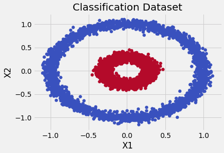
Assume that we’ve collected data and would like to build a new classifier. To be concrete, pretend that we’ve gathered up data where each sample has two variables, and an associated class label that tells us if it is a “blue dot” or a “red dot”. When we plot our data, we see a picture like this one:

Let’s formalize our notation a bit and represent each observation as a vector of 2 variables and convert our class labels of “blue” and “red” to a binary variable called , where and . Now we want to construct some function, let’s call it , to model the relationship between and so that when we get new data, we can correctly predict if it’s a blue dot or a red dot. The most straight-forward way to construct is weight each variable and add them up in a linear model:

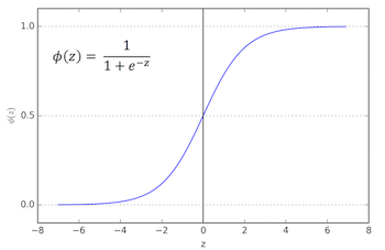
where each is a scalar that weights the contribution of each variable, and is the intercept term. So takes each variable, performs a weighted-sum to create a single real-valued number that we’d like to compare to our outcome variable, . Since our outcome is binary, we can’t directly compare it to , since our function can take on any number on the real line. Instead, we’ll transform so that it represents the probability . To do this we will need to introduce a function known as a logistic function, called :

represents the conditional probability that is a 1, given the observed values in , i.e. . This perhaps strange looking function takes the number created by and ‘squashes’ it be between 0 and 1, and gives us the conditional probability that we’re interested in. The graph of the sigmoid is shown below, with on the x-axis and on the y-axis:

Why should we prefer this specific function over potential alternatives? After all, there are many ways to squash a number to fall between 0 and 1. For one, it has a very nice and easy to compute derivate and it has a variety of nice statistical , yields interpretable quantities known as odds-ratios, but for now let’s just roll with it.

So we’ve defined a model , linked it to our target variable using the logistic function, and now we just have one more piece we need to define. We need a way to “measure” how close our predicted value, , is to the true value . This is known as a loss function, represented as . The most common choice for a loss function in a classification task like this is binary crossentropy (BCE), shown below: